If you follow fitness or nutrition research, you’ve probably heard the common phrase, “Correlation does not equal causation.” While this is true, it does not render all correlations meaningless. Correlations are commonly misinterpreted, which results in situations where people make leaps to unsupported conclusions, or miss out on important information by dismissing correlations altogether. But, with a little bit of background information about how correlations work, these common mistakes can be avoided.
What is a correlation?
Put simply, two values will be correlated if they vary together. For instance, consider height and weight. Taller people tend to weigh more, so weight goes up as height goes up. This is an example of a positive correlation, because the values vary in the same direction. You can also have a negative or inverse correlation, in which one variable goes down as the other goes up (e.g., the amount of weight you’re lifting, and the number of reps you can complete).
Let’s go back to the correlation between height and weight. This relationship may be true in general, but there are certainly cases of short people that are very heavy and tall people that are very light; these cases don’t follow the general pattern, which decreases the strength of the correlation. In most studies you see, the strength of the correlation between two variables is indicated by the Pearson product-moment correlation coefficient, denoted as R. This coefficient R can take any value ranging from -1 to 1. A weaker correlation results in an R value closer to 0, whether positive or negative (see Figure 1). Conversely, a stronger correlation results in an R value closer to -1 (strong negative correlation) or 1 (strong positive correlation). Correlations will also be reported with a p-value, which pertains to statistical significance. If the p-value is less than or equal to 0.05, correlations are generally considered “statistically significant,” which is a statistician’s way of saying that the R value of the correlation is reliable. P-values, which range from 0 to 1, can be interpreted as follows:
If we assume that there is no correlation between the two variables, and we get a p-value of 0.05, then we would expect to get a data set that indicates this strong or stronger of a correlation 5% of the time.
So, a low p-value increases your confidence that the variables actually are correlated.
What would happen if we looked at the correlation between height and weight in professional, stage-ready bodybuilders? Everyone is lean and everyone is muscular; compared to the general population, we would expect a stronger and more consistent relationship between height and weight. As a result, we would expect a higher R value and a lower p-value. To get an idea of how the direction and strength of correlations look graphically, check out this figure with some randomly generated data:
Figure 1. Strength and direction of correlations
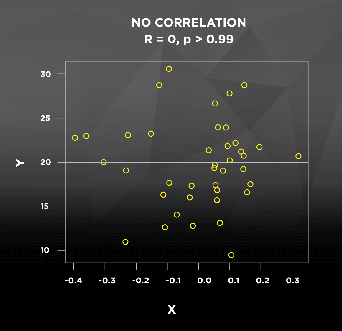
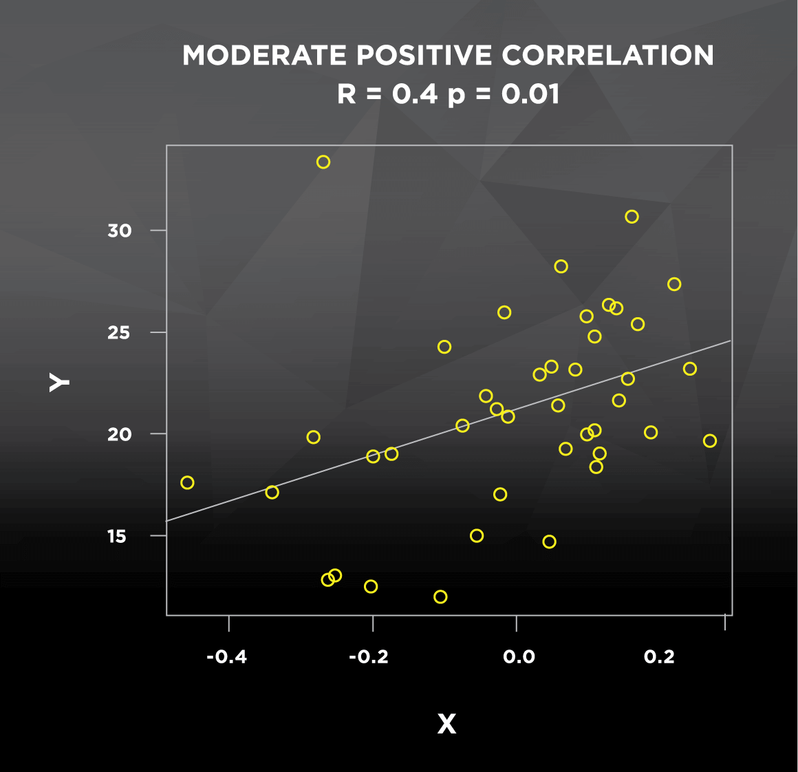
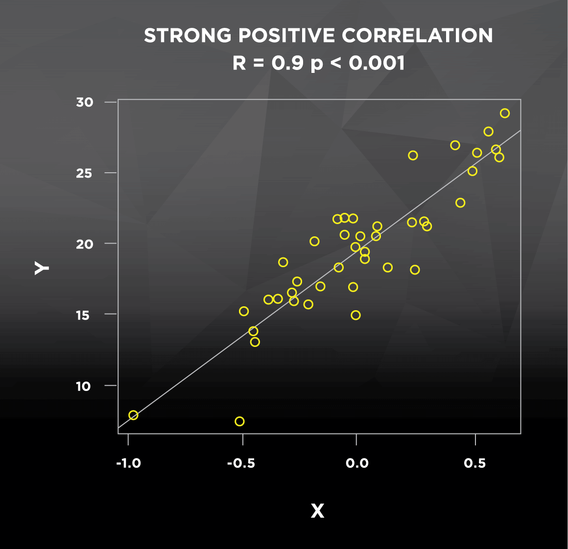
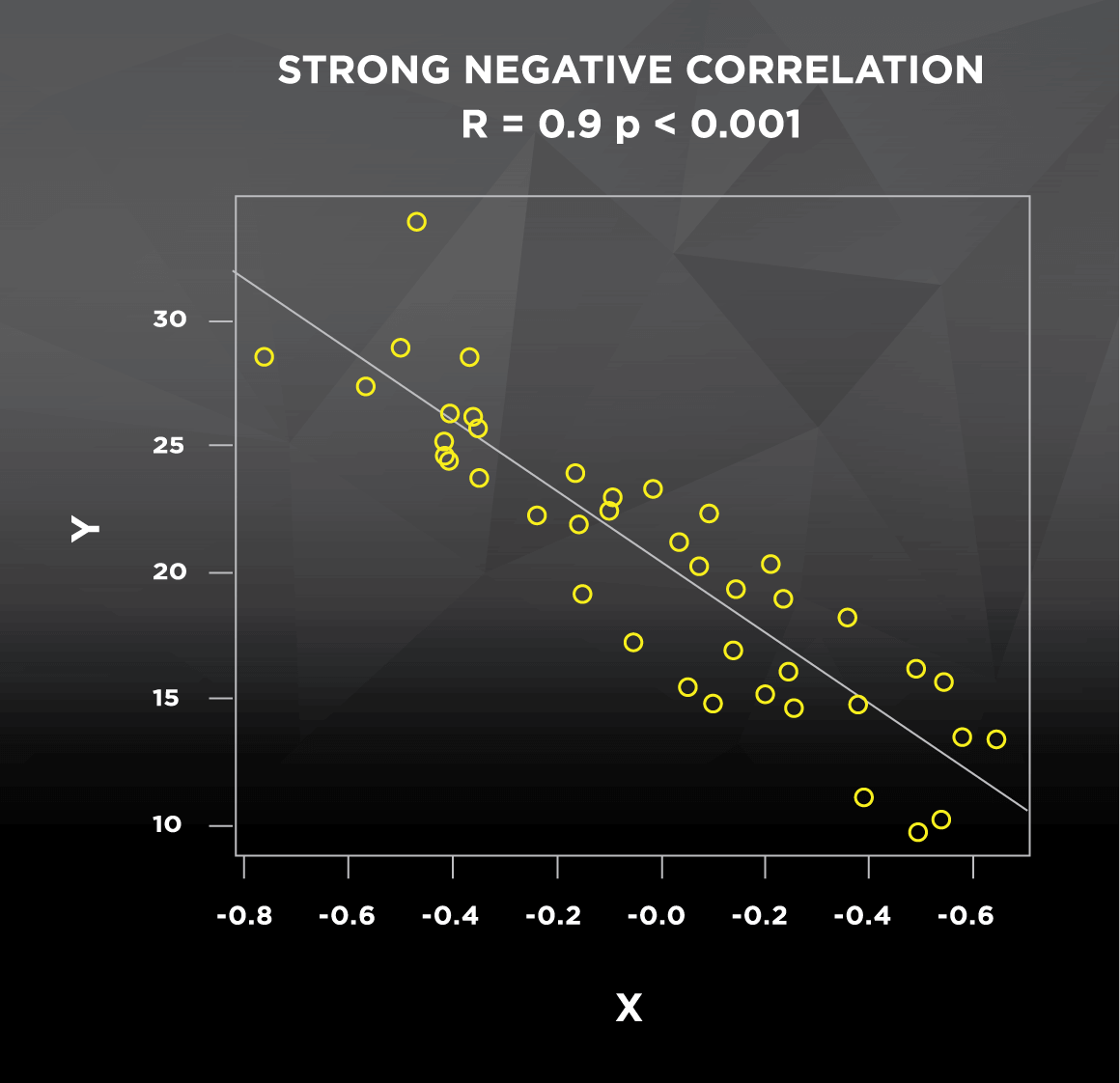
If you’ve ever seen the term regression used, it’s important to understand that some of the same information can be obtained from both correlation and regression. The lines in Figure 1 above are regression lines, also commonly known as lines of best fit that predict Y using X. The main difference between the two is that regression uses one variable to predict the other (How well does height predict weight?), while correlation assesses how they vary together (How do height and weight change in relation to each other?). This predictive application of regression explains how we can construct formulas to predict your metabolic rate based on height, weight, age, sex, etc. But at the end of the day, if I do a correlation between height and weight, or I use regression to predict weight using height, I will get the exact same R and p-values. Regression also returns an R2 value, which represents the proportion of the variability of Y (weight) that is explained by the X variable(s) in the model (height).
At this point, you can probably see that there’s value in the general idea of correlation. It helps us identify how consistently variables change together, which assists in identifying important patterns. Taken one step further, regression allows us to construct equations that predict one variable based on others. What’s even cooler is that regression is essentially the basis for the t-test and analysis of variance (ANOVA), which are comparison tests that some people erroneously consider superior to correlation and regression. A t-test is a special case of ANOVA, and ANOVA is a special case of regression. If you don’t believe me, check out result 1 (my t-test output) and result 2 (my regression output) below. I made up some bench press data to test if one group benches significantly more than another, and I tested it both ways. The highlighted values confirm that the t-test is exactly the same thing as regression when used here to determine how well group membership predicts bench press. If there were more than two groups, I would use ANOVA instead of a t-test, but regression would still give me the exact same result.
Result 1. T-test
data:  bench1 and bench2
t = -2.3273, df = 20, p-value = 0.03056
sample estimates:
mean of x mean of y
 278.8182  301.9091
Result 2. Regression
lm(formula = bench ~ group)

Coefficients:
            Estimate Std. Error t value Pr(>|t|)
(Intercept)  255.727     15.688  16.301 5.14e-13 ***
group         23.091      9.922   2.327   0.0306 *
---
Multiple R-squared:  0.2131,    Adjusted R-squared:  0.1738
F-statistic: 5.416 on 1 and 20 DF,  p-value: 0.03056
As you can see, regression is an extension of correlation, and t-tests/ANOVAs are special cases of regression. Bottom line: The general concept of correlation forms the basis for the statistical tests we use to evaluate relationships between variables. And while people sometimes diminish the value of correlations, in the following sections we’ll see that their meaning and value depend entirely on when and how they’re applied. There are innumerable cases in which well-conducted studies provide excellent evidence in the form of correlations. Nonetheless, correlations do have a couple major limitations that contribute to widespread misinterpretation.
1. Fairly meaningless correlations can be statistically significant
It’s important to realize that statistical significance has nothing to do with real-world significance. The most obvious examples of this are nonsensical correlations that occur randomly, such as the correlation between Nicolas Cage films per year and drowning rates [1]. In other cases, there is a confounding variable influencing the variables or the relationship between them. Imagine a correlation between monthly ice cream sales and drownings in Ohio; in this case, seasonal weather patterns would be a very obvious confounding variable. I’ve taken a few outdoor, late-November swims in Ohio, and I can assure you that they weren’t pleasant experiences.
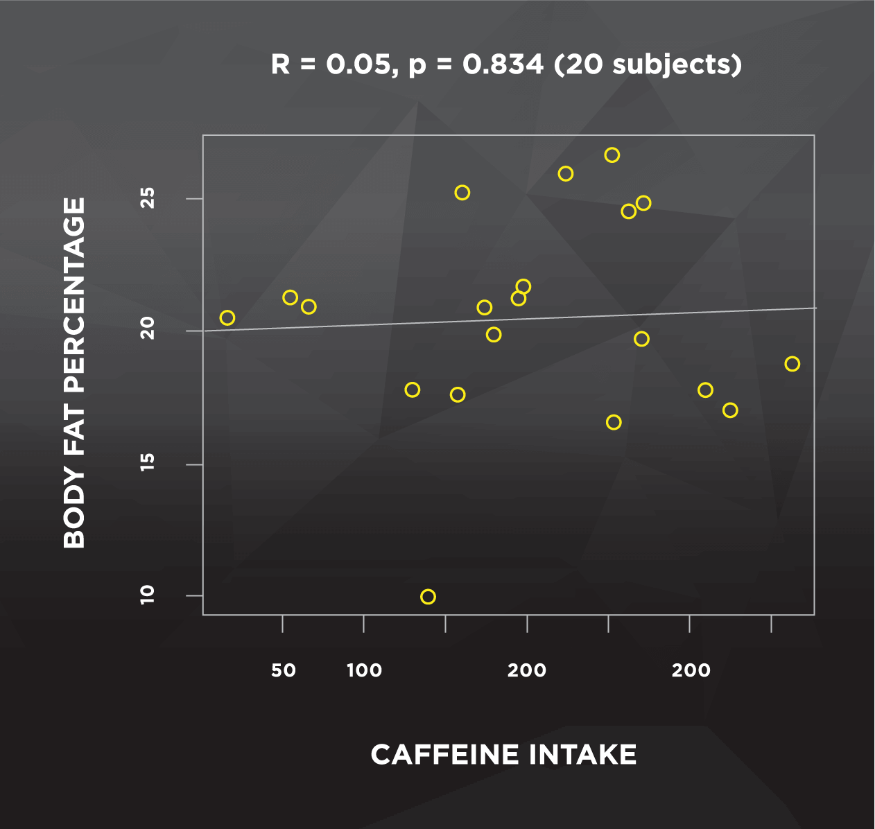
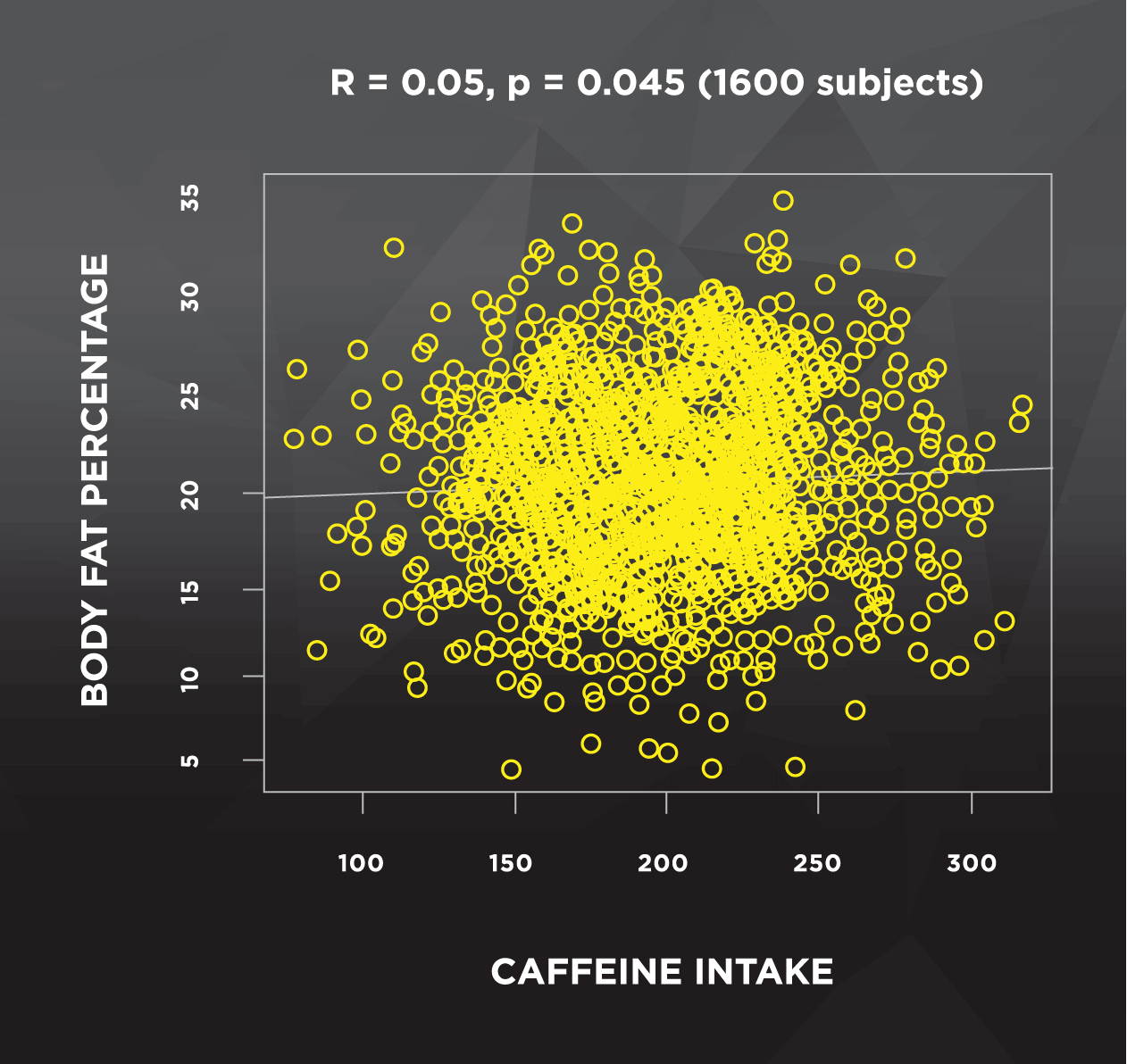
The final example for this point relates to studies with very large numbers of subjects. As sample size increases, it becomes more likely that small effects become statistically significant. I randomly generated two data sets to illustrate this point below. The left side of Figure 2 shows a sample with 20 subjects, and no clear pattern between body fat percentage and caffeine intake. The data on the right side were randomly generated using the same parameters, but using a sample of 1600 subjects instead of 20.
This situation can be tricky to interpret; both figures have the same correlation (R = 0.05), but only the large sample is statistically significant. Luckily, with correlations we can square the R value to help us out. Despite statistical significance, the R2 value is only 0.0025. This means that about one quarter of 1% of the variance of body fat percentage is explained by caffeine intake, which leaves the other 99.75% (essentially all of it) unexplained. We also see that the difference between the lowest and highest caffeine consumers is negligible– only about 1% body fat. For us to actually care, we’d want to see a reasonably high R2 value, and we’d need to see that a realistic increase in caffeine actually corresponds to a more substantial change in body fat percentage. So, this “significant” finding is pretty meaningless to us. Unfortunately, by the time this finding reaches the headlines, it’ll probably say “Shedding weight for that summer beach bod? Drop the coffee!” And you should never, ever drop the coffee.
Figure 2. Caffeine and body fat percentage: 20 subjects vs. 1600 subjects
2. Correlations don’t tell you what is causing the observed relationship
Let’s say a study administered a big survey and found that squat one rep max (1RM) was inversely correlated with long-distance running endurance. In this scenario, each of the following possibilities could be true, and we can’t be sure which is accurate:
Long-distance running causes a decrease in squat strength
Squatting impairs long-distance running endurance
There are other confounding variables that aren’t accounted for. One scenario might be that people who run a lot happen to spend less time squatting, and squat volume is the “true” variable dictating the relationship. This is plausible, but the number of possibilities is virtually endless
People often attribute this shortcoming to correlation tests, but it’s more so an issue of study design. The general concept of correlation is highly valuable, but correlational designs are inherently limited. Correlational designs are a type of non-experimental study design, meaning the researchers have little to no control over the variables of interest– they just observe. The researchers haven’t controlled anything, so they can’t say if X caused Y, Y caused X, or if some other variable(s) are affecting the relationship. Experimental designs are just the opposite– researchers randomly assign groups, apply an intervention, control as many confounders as possible, and can make a strong case for causation. In correlational designs, researchers will frequently make mathematical adjustments to their correlation/regression models, in an attempt to account for potential confounding variables. These adjustments are helpful, but they fall short of truly controlling the variables at hand.
With this in mind, the context of a correlation is critical. If researchers report a correlation between two variables with no justifiable connection (e.g. Nicolas cage movies and drowning), you’d have huge doubts about how valuable that information is. If they report a justifiable correlation without controlling for obvious confounding variables, you’d still have major concerns. On the other end of the spectrum, imagine that researchers report a correlation with a plausible explanation and run a regression on the data that returns a decently high R2 value, using a model that is appropriately adjusted for confounders. While we still can’t be certain of what is causing the observed relationship, this type of correlation or regression model would provide fairly compelling evidence. In some cases, this evidence could then be used to justify a new study, this time with an experimental design that has the ability to rigorously investigate a possible causal relationship.
Finally, imagine researchers wanted to see if carbohydrate intake affects maximal, high-intensity exercise performance. So they recruited subjects, kept them in a metabolic ward, and controlled everything possible (diet, physical activity, sleep, etc.). The day before the exercise bout, they randomly assigned subjects to a low carb, medium carb, or high carb diet, with equal calories and protein. The researchers determined that high was better than medium, and medium was better than low. If they wanted to, they could evaluate the role of muscle glycogen content by splitting the sample into “high glycogen” and “low glycogen” groups, and using a t-test to compare them. An alternative strategy would be to evaluate the correlation between muscle glycogen content and performance. Let’s say they chose the latter, with results indicating a significant correlation between pre-exercise muscle glycogen content and performance. Despite being “just a correlation,” this particular correlation represents very strong evidence, based on the tightly controlled study design.
On the other hand, let’s say I bring in 30 males for one lab visit, and I measure their bench press and testosterone levels. I could use a correlation test to see that there was a positive correlation between testosterone and bench press, but I can’t say which variable “caused” the relationship. I could also split them into low-testosterone and high-testosterone groups, and use a t-test to see that the high testosterone group benched more than the low group. Some people might argue that these results suggest that higher testosterone levels caused higher bench press numbers, because it’s a t-test instead of a correlation. And they’re dead wrong.
Despite the use of a t-test, they cannot argue for causation based on the study design. They didn’t control their training, nutrition, testosterone, or anything else, so how could they know that testosterone actually caused the difference? Compared to the previous example of muscle glycogen content and performance, we see an instance in which correlations can actually yield stronger evidence than a t-test, based on how the study was designed. So when people say “Correlation doesn’t equal causation,” this statement says a lot more about study design than it does about the statistical test employed.
Conclusions
Correlational study designs are neither bad nor useless. They allow us to identify patterns that guide future experimental research, allow us to investigate research questions before spending the time and resources to run a controlled study, and help us investigate research questions that would be unethical to study in humans. No one is going to force a group of people to consume a suspected carcinogen and see if they develop cancer, but they can certainly observe people who already consume the suspected carcinogen. In addition, the mathematical concept of correlation forms the backbone for many of the statistical tests that are used today. However, statistical tests are tools we use to guide and organize thinking, not a replacement for thinking. This means that correlations must be carefully evaluated based on their study design, context, sample size, real-world significance, and plausibility. So no, correlation does not mean causation. But it doesn’t mean “worthless,” either.
References
Co-written by Sarah Reifeis
Sarah Reifeis is a PhD student at UNC Chapel Hill in the Department of Biostatistics. She currently works as a research assistant for the Biostatistics Core of the UNC Center for AIDS Research, where she provides statistical consulting and analysis for HIV/AIDS researchers at UNC. Sarah completed her bachelor’s degree in mathematics at Indiana University in 2015, where she also conducted research in chemistry and worked as a teaching assistant for various biology courses.

